Play with embedding using SmooSense on MacBook Pro

Embeddings are quietly powering almost every AI feature you use — from image search and recommendation to retrieval-augmented generation and multimodal reasoning. They convert complex objects (like images or text) into compact numerical vectors that capture semantic meaning.

Most people assume that playing with embeddings requires data-center GPUs, clusters, and large cloud bills. But here’s the good news: you don’t need any of that to get started.

If you have a MacBook Pro with an M-series chip, you already own a surprisingly capable AI workstation. Pair it with SmooSense, our lightweight visual data playground, and you can explore, visualize, and compare embeddings interactively — all within your laptop.

1. Why MacBook Pro is secretly powerful for embeddings#

Apple’s M-series chips (like M4 Pro or M3 Max) integrate high-bandwidth unified memory, efficient matrix cores, and the MPS backend (Metal Performance Shaders) for PyTorch. That means you can run modern embedding models (like CLIP, SigLIP, DINOv2) directly on the Mac GPU in half precision (fp16) — no CUDA, no setup.

Typical speed-ups:

So instead of waiting for cloud instances to spin up, you can compute embeddings in real time while sipping coffee.

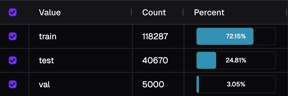
2. Verifying Dataset Balance with SmooSense#

In machine learning dataset curation, one of the most critical quality checks is data balance — ensuring that your training, validation, and test splits represent similar distributions. For categorical or numeric metadata, this is straightforward: a few SQL queries will do.

However, when you want to verify balance in semantic space — for example, whether your training and validation sets cover the same range of visual styles, scenes, or embeddings — things get harder. Traditional plots or summary tables fail to capture the high-dimensional structure that embeddings encode. Now we introduce an intuitive and scalable way using SmooSense.

Here we use COCO dataset as the example.

2.1 Step 1. compute embeddings (163,957 images in 14 minutes)#

Just vibe-code a python script to compute CLIP embedding with MPS acceleration, and then save to parquet file locally. Below is a reference.

# pip install open_clip_torch torch torchvision pillow pyarrow pandas tqdm umap-learn
import os

import numpy as np
import open_clip
import pandas as pd
import torch
from PIL import Image
from torchvision.transforms import v2 as T
from tqdm import tqdm

# ------------------- config -------------------
DATA_DIR = os.path.expanduser('~/Work/COCO2017')
INPUT_PARQUET = os.path.join(DATA_DIR, 'organized/images.parquet')
OUTPUT_PARQUET = os.path.join(DATA_DIR, 'organized/images_with_embeddings.parquet')
MODEL_NAME, PRETRAINED = "ViT-B-32", "openai"
BATCH_SIZE = 128          # try 64–256 on M4
EMB_DIM = 512             # 768 for ViT-B/16 etc.
# ------------------------------------------------

device = torch.device("mps" if torch.backends.mps.is_available() else "cpu")
print(f"Using device: {device}")

# Load model + preprocess
print("Loading model...")
model, _, preprocess = open_clip.create_model_and_transforms(
    MODEL_NAME, pretrained=PRETRAINED, device=device
)
model.eval()
amp_dtype = torch.float16

# Image transforms
to_tensor = T.Compose([
    T.Resize(256, interpolation=T.InterpolationMode.BICUBIC),
    T.CenterCrop(224),
    T.ToImage(),
    T.ToDtype(torch.float32, scale=True),
    T.Normalize(mean=[0.48145466, 0.4578275, 0.40821073],
                std=[0.26862954, 0.26130258, 0.27577711]),
])

# Load data
print("Loading parquet file...")
df = pd.read_parquet(INPUT_PARQUET)
print(f"Total rows: {len(df)}")

# Prepare embeddings list
embeddings = []

# Process in batches
with torch.inference_mode(), torch.autocast(device_type="mps", dtype=amp_dtype):
    for idx in tqdm(range(0, len(df), BATCH_SIZE), desc="Computing embeddings"):
        batch_df = df.iloc[idx:idx+BATCH_SIZE]
        batch_tensors = []

        for _, row in batch_df.iterrows():
            image_path = os.path.join(DATA_DIR, f"{row['fold']}2017", row['file_name'])
            img = Image.open(image_path).convert("RGB")
            x = to_tensor(img)
            batch_tensors.append(x)

        # Stack batch and move to device
        x_batch = torch.stack(batch_tensors).to(device, non_blocking=True)
        x_batch = x_batch.to(dtype=amp_dtype, memory_format=torch.channels_last)

        # Compute embeddings
        feats = model.encode_image(x_batch)
        feats = torch.nn.functional.normalize(feats, dim=-1)

        # Convert to numpy
        feats = feats.to("cpu", dtype=torch.float32).numpy()
        embeddings.extend(feats.tolist())

# Add embeddings column to dataframe
df['emb'] = embeddings

# Save to parquet
print(f"Saving to {OUTPUT_PARQUET}...")
df.to_parquet(OUTPUT_PARQUET, compression='zstd', index=False)

After testing with small batch, we can run the script for all images.

We can also open "Activity Monitor", go to Menu -> Windows -> GPU history and verify if it is really using GPU.

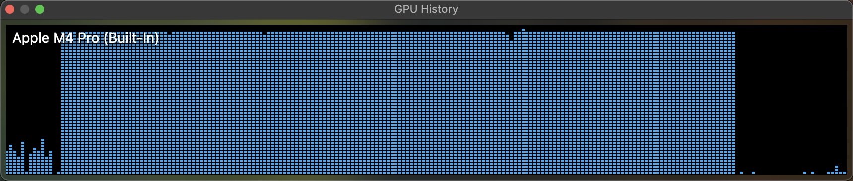
On my laptop, it took 14 minutes to process 164k images, roughly 195 images per second. Since I bought the cheapest tier of MacBook Pro M4, it is expected to be in the lower side of the range. Still, this is very impressive for a laptop. It gives almost-zero overhead and fast iterations to work with small and medium size datasets.

2.2 Reduce embedding dimension (512 => 2)#

To help humans see structure in embedding data, we must project those high-dimensional vectors into 2D while keeping their neighborhood relationships intact. UMAP (Uniform Manifold Approximation and Projection) is one of the most popular algorithms. At its core, UMAP tries to preserve the local geometry of the data — meaning that points that are close in the original embedding space stay close after projection, while distant points remain separate.

import umap

# Compute UMAP 2D projection
print("Computing UMAP projection...")
embeddings_array = np.array(embeddings)
reducer = umap.UMAP(n_components=2, random_state=42, n_neighbors=15, min_dist=0.1)
umap_coords = reducer.fit_transform(embeddings_array)

# Add UMAP coordinates to dataframe
df['emb_x'] = umap_coords[:, 0]
df['emb_y'] = umap_coords[:, 1]

2.3 Visual exploration using SmooSense BalanceMap#

To make large-scale embedding data intuitive and explorable, we introduce BalanceMap — a visualization designed for both scalability and insight.

2.3.1 Scalable bubble-based visualization

Instead of plotting every point individually, BalanceMap aggregates nearby data points into bubbles, where each bubble represents a local cluster in the embedding space.

The bubble size reflects the number of points it contains, providing a clean, high-level view even when dealing with billions of data points.

This approach preserves spatial structure while eliminating visual clutter.

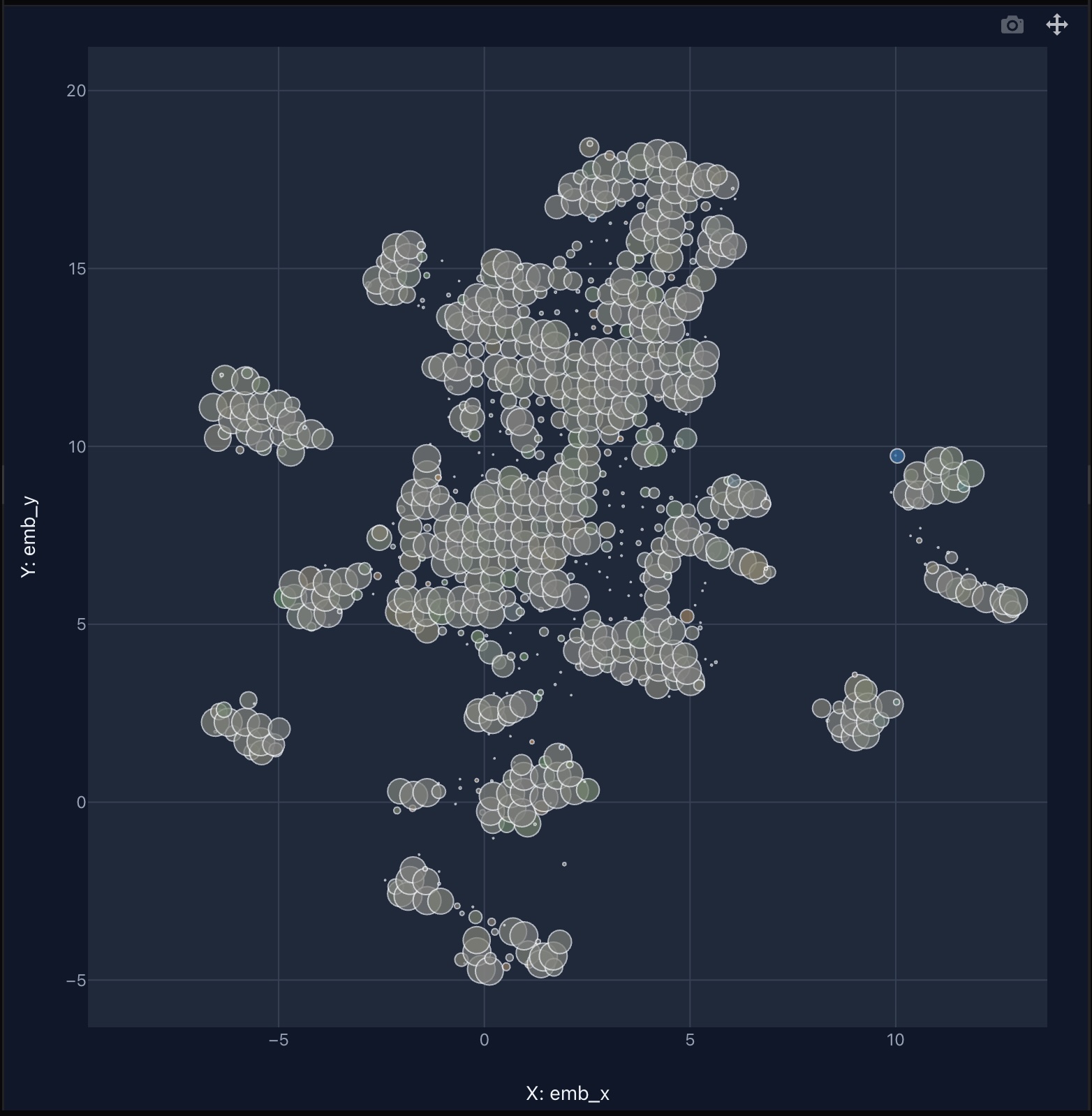
2.3.2 Ratio-based color encoding for balance

Color isn't determined by raw counts, but by relative balance across breakdowns (e.g., training/validation/test splits). This is because groups of the breakdown inherently have different size. Image below shows the distribution of fold. If we colorize by counts, then you will only see information from training fold.

For each bubble, we compute the ratio of samples of that bubble within its breakdown group:

$\text{ratio} = \frac{\text{count of points in bubble}}{\text{count of total points in that group}}$

We then compare these ratios across groups:

Example of good balance. When ratios are equal, the bubble is colored with neutral gray, indicating balance. Hovering on bubble will show detailed counts and ratios.

Example of imbalance. When ratios differ, the color shifts toward the dominant group, making imbalances immediately visible.

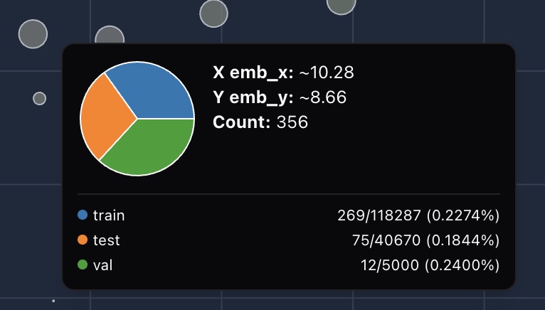
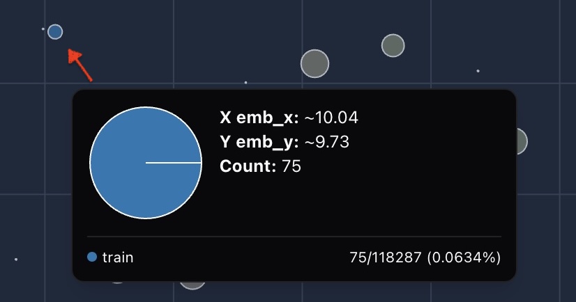
This ratio-based coloring highlights subtle dataset skews that simple count comparisons would miss.

2.4 Automated sampling#

Clicking on a bubble opens a gallery view of representative samples, allowing quick qualitative inspection without leaving the map.

2.5 Breakdown with other metadata#

What if you want to check balance for other categorical columns? Simply change the breakdown column and then you get it.

In the example below, we first click the license treemap in left side bar to change it to categorical, and then change "Breakdown column" to license. Combining bubble

3. Takeaways#

• MacBook Pro is a powerful local lab. Its built-in M-series GPU can accelerate embedding computation by up to 8×, making it perfectly capable of running quick experiments on datasets of up to one million images — all without external infrastructure.
• Visualization is key to understanding embeddings. To make sense of high-dimensional data, we need intuitive visual tools that reveal structure, bias, and distribution — not just numbers.
• SmooSense BalanceMap turns embeddings into insight. It transforms massive embedding datasets into a clear, interactive landscape, where data balance becomes something you can literally see.